Bayesian inference primer: local curvature
Local curvature goes by many names in the literature: the Fisher information matrix, the Laplace approximation, the Gaussian approximation. They all refer to the same idea: replace complicated formulas with simple ones by approximating a distribution by its mode centered around a (multivariate) normal distribution. To understand how this works, note that much intuition around Bayesian inference can come from the linear regression, which takes in a set of labeled data, each containing a feature a vector x and an output y, and learns a set of weights θ for each dimension of x plus and intercept that minimizes some cost function between the labels y and the dot product between the weights and the feature vector, plus the intercept. We use this model as a standard candle because there is a closed-form solution we can use to compare against other numerical methods.
One such method uses the curvature of the likelihood function at the maximum a posteriori (that is, the global optimum of the likelihood function). Because linear regression is a convex problem, we can use gradient ascent on the likelihood function to find its global optimum and guarantee that it is global. But what is the spread of the density of the likelihood function around it?
For this problem, it turns out that we can use the curvature of the likelihood function at its global maximum to derive an exact solution that matches the closed-form solution. How do we calculate it? We start with the likelihood function
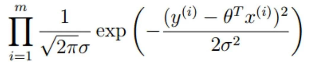
where we compute the product over m data points. The negative log-likelihood function is then proportional to the sum of squared distances between the y values and the model predictions, that is, the residuals. Welcome to ordinary least squares!
All this math means that if we take the second derivative of the negative log-likelihood with respect to the model parameters θ, that is, the Hessian matrix, and invert it, we get the covariance matrix of our model parameters. And because we can prove this, it means that any numerical method for calculating partial derivatives can be applied and work equally well. Even better, there are additional mathematical identities (cue in the Jacobian) that allow us to use different numerical approaches to calculate the same thing and ensure stability.
For the linear regression, of course, this is all overkill, but even in this humble model using the local curvature, can provide some big wins. For example, an iterative algorithm allows us to train a Bayesian linear or logistic regression with only a diagonal covariance matrix, which means that the number of parameters we need to update grows linearly rather than quadratically with the number of features, a huge boon for industrial applications with large dimensionality. Moreover, it makes the Bayesian logistic regression for making binary predictions feasible, even though Bayesian inference is usually intractable in this case. For more complex models, employing local curvature can be a life-saver, since, if we can numerically calculate the derivatives, then we’re in business. It even forms the basis of the most successful approaches in variational inference.
Common tools for performing this calculation in python include:
Certain optimization algorithms within the scipy optimize function use the Hessian to find the maximum likelihood estimate, and can return those values for your use. See
The numdifftools library is a popular choice for numerically calculating derivatives.
If you want to get really fancy, and use the slick tools adopted by Google’s DeepMind, you can use JAX.
There are pros and cons to each approach for calculating these derivatives. However, note that in our experience, the numerical approaches often have large caveats and may never converge. The JAX solution is a sort-of-symbolic approach that only yields to certain types of models that can be encoded using its library of Python functions. In other words, except for canonical models like the ones discussed in this article, the Laplace approximation isn’t automatable without helper libraries which are still in development and may not always work, for example, in models that require simulations to relate the parameters to the output. This means that we are still looking for better ways to perform Bayesian inference.
Code sample for local curvature
# Using Least Squares

import scipy as sp
results = sp.optimize.least_squares(error_function,
                                    initial_parameters,
                                    bounds=bounds)

parameters_at_maximum_likelihood = results.x
hessian = results.jac.T @ results.jac
covariance_matrix = np.linalg.inv(hess)

# Using Curve Fit

import scipy as sp
parameters_at_maximum_likelihood, covariance_matrix = \
  sp.optimize.curve_fit(curve_fit_func,
                        x_data,
                        y_data,
                        p0=initial_parameters,
                        bounds=bounds)

# Using numdifftools

import scipy as sp
import numdifftools
import numpy as np
results = sp.optimize.minimize(-log_likelihood_function,
                               initial_parameters,
                               bounds=bounds,
                               method=method_string)
parameters_at_maximum_likelihood = results.x
if hasattr(results, 'hess_inv'):
    covariance_matrix = results.hess_inv
else:
    hessian_matrix = numdifftools.Hessian(log_likelihood_function)(parameters_at_maximimum_likelihood)
    covariance_matrix = cov = np.linalg.inv(-hess)
Outline of the Bayesian inference primer
Bayesian inference methods:
Bayesian linear regression
Gaussian processes
Bayesian neural nets (BNNs)